04 Best response polytopes

Corresponding chapters

• Best response polytopes

Objectives

• Define the best response polytopes (using both definitions: convex hull and halfspaces).
• Labelling of vertices
• Equivalence between equilibrium and fully labeled pair
• Vertex enumeration

Notes

Defining best response polytopes

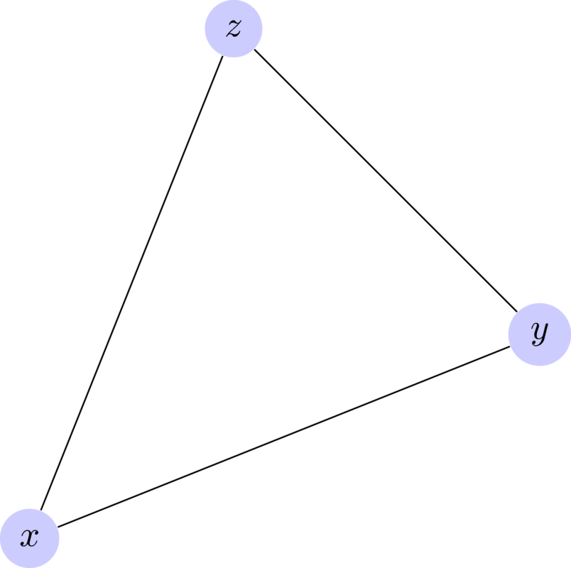
Discuss what an average is. Place this in the context of the line between two points. Weighted averages of two points are just a line. So an average is just a probability distribution. Expand this notion to the average over two points. How would you take the weighted average between three points \(x, y, z\):

\[\lambda_1 x + \lambda_2 x + \lambda_3 x\]

This corresponds to something like:

Explain how another definition for that space would be draw inequalities on our variables. Give definition of best response polytopes for a game. Illustrate this with the battle of the sexes game (scaled!):

\[\begin{split}A = \begin{pmatrix} 3 & 1\\ 0 & 2\\ \end{pmatrix} \qquad B = \begin{pmatrix} 2 & 1\\ 0 & 3\\ \end{pmatrix}\end{split}\]

Go over the definition of the best response polytopes.

The row best response polytope is given by:

\[\mathcal{P} = \left\{x\in\mathbb{R}^{m}\;|\;x\geq 0; xB\leq 1\right\}\]

This corresponds to the following inequalities:

• \(x_1\geq 0\)
• \(x_2\geq 0\)
• \(2x_1\leq 1\)
• \(x_1+3x_2\leq 1\)

From this we can identify the vertices:

• \((x_1, x_2)=(0,0)\)
• \((x_1, x_2)=(1/2,0)\)
• \((x_1, x_2)=(0,1/3)\)
• \((x_1, x_2)=(1/2,1/6)\)

This can be confirmed using nashpy:

>>> import numpy as np
>>> import nash
>>> B = np.array([[2, 1], [0, 3]])
>>> halfspaces = nash.polytope.build_halfspaces(B.transpose())
>>> for v, l in nash.polytope.non_trivial_vertices(halfspaces):
...     print(v)
[ 0.5  0. ]
[ 0.          0.333...]
[ 0.5         0.166...]

The column best response polytope is given by:

\[\mathcal{Q} = \left\{y\in\mathbb{R}^{m}\;|\;Ay\leq 1; y\geq 0\right\}\]

This corresponds to the following inequalities:

• \(3y_1+y_2\leq 1\)
• \(2y_2\leq 1\)
• \(y_1\geq 0\)
• \(y_2\geq 0\)

From this we can identify the vertices:

• \((y_1, y_2)=(0,0)\)
• \((y_1, y_2)=(1/3,0)\)
• \((y_1, y_2)=(0,1/2)\)
• \((y_1, y_2)=(1/6,1/2)\)

Confirmed:

>>> import numpy as np
>>> import nash
>>> A = np.array([[3, 1], [0, 2]])
>>> halfspaces = nash.polytope.build_halfspaces(A)
>>> for v, l in nash.polytope.non_trivial_vertices(halfspaces):
...     print(v)
[ 0.333...  0.        ]
[ 0.   0.5]
[ 0.1666...  0.5       ]

Pair activity

Ask everyone to draw these two polytopes.

Now describe how we label the vertices: using the same ordering as the inequalities (starting at 0), a vertex has the label corresponding to that inequality if it is a strict equality.

\(\mathcal{P}\):

\(\mathcal{Q}\):

Explain that what these polytopes represent is the scaled strategies when players maximum utilities are 1. So given, the action of an opponent, if the players’ utility is 1 they are playing a best response.

Ask students to assign each other either \(\mathcal{P}\) or \(\mathcal{Q}\). Both players should choose a vertex and investigate the utilities.

For example, if:

• The row player (\(\mathcal{P}\)) picked: \((0, 1/3)\) with labels: \(\{0, 3\}\).
• The column player (\(\mathcal{Q}\)) picked: \((1/6, 1/2)\) with labels: \(\{0, 1\}\).

This implies:

• The row player is not playing their first strategy (label 0), so playing their second strategy. Also (label 3), the best response to this is that the column player plays their second strategy.
• The best response to what the column player is currently doing is to play both strategies.

At this point the column player has an incentive to move, they will move to the \((0, 1/2)\) vertex with labels: \(\{1, 2\}\) which implies:

• The row player is as before.
• The column player is playing their first strategy (label 2). The best response to this is for the row player to play their second strategy (label 1).

So this is a Nash equilibria.

Another example:

• The row player (\(\mathcal{P}\)) picked: \((1/2, 1/6)\) with labels: \(\{2, 3\}\).
• The column player (\(\mathcal{Q}\)) picked: \((1/6, 1/2)\) with labels: \(\{0, 1\}\).

This implies:

• The best response to what the row player is currently doing is to play both strategies.
• The best response to what the column player is currently doing is to play both strategies.

Neither player has a reason to move.

Another example:

• The row player (\(\mathcal{P}\)) picked: \((0, 1/3)\) with labels: \(\{0, 3\}\).
• The column player (\(\mathcal{Q}\)) picked: \((1/3, 0)\) with labels: \(\{0, 3\}\).

This implies:

• The row player is not playing their first strategy (label 0), so playing their second strategy. Also (label 3), the best response to this is that the column player plays their second strategy.
• The column player is not playing their second strategy (label 3), so playing their first strategy. Also (label 0), the best response to this is that the row player plays their first strategy.

Neither player is happy here. Once one moves (not allowing the origin because that’s not playing) we arrive at a similar situation to before.

After students have walked through this themselves have a discussion about what property seems to indicate Nash equilibrium. Move to discussing the notes.

In particular highlight that we’ve scaled the utility so we need to (at the end) scale the vertices too!

Finally show how this is implemented in nashpy:

>>> A = np.array([[1, -1], [-1, 1]])
>>> matching_pennies = nash.Game(A)
>>> for eq in matching_pennies.vertex_enumeration():
...     print(eq)
(array([ 0.5,  0.5]), array([ 0.5,  0.5]))